Unit outcomes

By the end of this unit you will be able to:

• Define a function.
• Identify if a relationship is a function or not.
• Sketch and find the equation of a linear function ([latex]\scriptsize y=ax+q[/latex] or [latex]\scriptsize y=mx+c[/latex]).
• Explain the effects on the shape of the graphs of linear functions of [latex]\scriptsize a[/latex] and [latex]\scriptsize q[/latex] or [latex]\scriptsize m[/latex] and [latex]\scriptsize c[/latex].
• Find the equation of a linear function from its graph or other details.
• State the domain and range of a linear function.

What you should know

Before you start this unit, make sure you can:

• Manipulate and simplify algebraic expressions. Go over Subject outcome 2.2, Unit 1: Simplifying algebraic expressions if you need more help with the basics.
• Solve linear equations. Go over Subject outcome 2.3, Unit 1: Solve linear and quadratic equations if you need more help with the basics.
• Plot points on the Cartesian plane.

Here is a short self-assessment to make sure you have the skills you need to proceed with this unit.

Solve for [latex]\scriptsize x[/latex] in each case.

1. [latex]\scriptsize 5x=2x+45[/latex]
2. [latex]\scriptsize -7x=8(1-x)[/latex]
3. [latex]\scriptsize \displaystyle \frac{1}{5}(x-1)=\displaystyle \frac{1}{3}(x-2)+3[/latex]

Solutions

1. .
   [latex]\scriptsize \begin{align*} 5x&=2x+45 \\ \therefore 3x&=45 \\ \therefore x&=15 \end{align*}[/latex]
2. .
   [latex]\scriptsize \begin{align*} -7x&=8(1-x) \\ \therefore -7x&=8-8x \\ \therefore x&=8 \end{align*}[/latex]
3. .
   [latex]\scriptsize \begin{align*} \displaystyle \frac{1}{5}(x-1)&=\displaystyle \frac{1}{3}(x-2)+3 \\ \therefore 3(x-1)&=5(x-2)+45 \\ \therefore 3x-3&=5x-10+45 \\ \therefore -2x&=38 \\ \therefore x&=-19 \end{align*}[/latex]

Introduction

Functions are one of the primary reasons mathematics is so important and useful. Functions let us describe and explore the relationships between different quantities. This in turn helps us design and build real things like buildings, planes, computers, and cell phones. Once we can explore the relationship between things, we can use this information to predict changes in populations and the economy, and even fight diseases like cancer and HIV.

Functions

What is a function?

Before we can start working with linear functions, we need to know what functions are. Let’s start with an activity.

Activity 1.1: What is a function?

Time required: 45 minutes

What you need:

• a pen or pencil
• four bottle tops and jar lids
• a ruler
• string
• a calculator
• blank paper or a notebook

What to do:

1. Collect four bottle tops and jar lids of different sizes (so circles of different sizes). Now, carefully use your ruler to measure the diameter of each top or lid (that is the straight-line distance from one side to the other through the centre). Use a piece of string to measure the circumference (the distance around the outside edge of each top or lid) by tightly wrapping the string around the lid and then measuring the length of string needed to go once all the way around.

NOTE: If you cannot get real lids, then just draw a few circles of different sizes on a piece of paper using a compass.

Record your measurements for each top or lid in a table like this one:

	Lid 1	Lid 2	Lid 3	Lid 4
Diameter
Circumference
[latex]\scriptsize \displaystyle \frac{\text{circumference}}{\text{diameter}}[/latex]

In the last row, calculate the circumference divided by the diameter for each lid to 2 decimal places.

Now answer these questions:

1. 1. What do you notice about your answers?
   2. Do you recognise this number? What number is it?
   3. If you know the diameter of a lid, how could you predict its circumference? Why?
   4. Write an equation that shows the relationship between the circumference and diameter.
   5. If the diameter of a certain lid is [latex]\scriptsize 12~\text{cm}[/latex], what is its circumference?
   6. If the circumference of a certain lid is [latex]\scriptsize 15.24~\text{cm}[/latex], what is its diameter?
   7. If you know the diameter is there any chance that there is more than one corresponding circumference?
2. Now look at the partly completed table of values in Table 1. The values have been generated using the equation [latex]\scriptsize y=\pm \sqrt{25-x^2}[/latex]. This just so happens to be the equation of a circle with a radius of five units and its centre on the origin of the Cartesian plane.

Table 1: Table of values of [latex]\scriptsize x[/latex] and [latex]\scriptsize y[/latex] related by the equation [latex]\scriptsize y=\pm \sqrt{25-x^2}[/latex]

Values of [latex]\scriptsize x[/latex]	-5	-4	-3	-2	-1	0	1	2	3	4	5
Values of [latex]\scriptsize y[/latex]	0		[latex]\scriptsize \pm4[/latex]	[latex]\scriptsize \pm4.58[/latex]						[latex]\scriptsize \pm3[/latex]

1. 1. Complete the table (rounding your answers off to two decimal places where necessary).
   2. Does every value of [latex]\scriptsize x[/latex] correspond with only a single value of [latex]\scriptsize y[/latex]?
   3. Draw your own circle with a radius of five units and its centre on the origin of a Cartesian plane. Why do you think each value of [latex]\scriptsize x[/latex] is associated with more than one value of [latex]\scriptsize y[/latex]?

What did you find?

In Question 1, you measured the diameter and circumference of various differently-sized lids. You should have noticed that all the answers in the bottom row of your table were about [latex]\scriptsize 3.14[/latex]. In other words, in each case, the circumference was about [latex]\scriptsize 3.14[/latex] times greater than the diameter. Table 2 shows the values someone measured.

Table 2: Completed table of the measurement of the diameters and circumferences of various lids

	Lid 1	Lid 2	Lid 3	Lid 4
Diameter	[latex]\scriptsize 2~\text{cm}[/latex]	[latex]\scriptsize 2.4~\text{cm}[/latex]	[latex]\scriptsize 5.2~\text{cm}[/latex]	[latex]\scriptsize 10.7~\text{cm}[/latex]
Circumference	[latex]\scriptsize 6.3~\text{cm}[/latex]	[latex]\scriptsize 7.5~\text{cm}[/latex]	[latex]\scriptsize 16.4~\text{cm}[/latex]	[latex]\scriptsize 33.9~\text{cm}[/latex]
[latex]\scriptsize \displaystyle \frac{\text{circumference}}{\text{diameter}}[/latex]	[latex]\scriptsize 3.15[/latex]	[latex]\scriptsize 3.13[/latex]	[latex]\scriptsize 3.15[/latex]	[latex]\scriptsize 3.14[/latex]

We can see that all the answers are more or less the same and that they are all about [latex]\scriptsize 3.14[/latex]. You might know that this number is an estimate of pi ([latex]\scriptsize \pi[/latex]).

Because the ratio of the length of the circumference to the diameter of a circle is a constant number, we can use this to predict the circumference of any lid if we know its diameter.

We can say that [latex]\scriptsize \displaystyle \frac{\text {circumference}}{\text {diameter}}\approx 3.14[/latex]. Therefore, [latex]\scriptsize {\text {circumference}}\approx {\text {diameter}}\times 3.14[/latex]. So, if the diameter is 12 cm, the circumference will be [latex]\scriptsize {\text {circumference}}\approx 12\times 3.14 =37.68\text{cm}[/latex].

If we know that [latex]\scriptsize \displaystyle \frac{\text {circumference}}{\text {diameter}}\approx 3.14[/latex], we can also say that [latex]\scriptsize \displaystyle \frac{\text {circumference}}{3.14}\approx \text{diameter}[/latex] . So, if the circumference is [latex]\scriptsize 15.24~\text{cm}[/latex], the diameter will be diameter [latex]\scriptsize \approx \displaystyle \frac{\text {circumference}}{3.14}=\displaystyle \frac{15.24\text{cm}}{3.14}=4.85\text{cm}[/latex].

For every diameter (or circumference), there is only one size of circle that can exist so there is only one corresponding circumference (or diameter). We can see from the equation [latex]\scriptsize \displaystyle \frac{\text {circumference}}{\text {diameter}}\approx 3.14[/latex] that no matter what diameter we put into the equation, we will only ever get one answer for the circumference.

In Question 2, you used the equation for a circle of radius five units and centre on the origin of the Cartesian plane ([latex]\scriptsize y=\pm\sqrt{25-x^2}[/latex]) to complete a table of values.

You should have seen that for every value of [latex]\scriptsize x[/latex] we feed into the equation, we get two values of [latex]\scriptsize y[/latex] out of the equation (except for when [latex]\scriptsize x=-5[/latex] or [latex]\scriptsize x=5[/latex]).

If we draw a circle of radius five units with its centre on the origin of the Cartesian plane, we get Figure 1.

Looking at Figure 1, we can see why each value of [latex]\scriptsize x[/latex] that we put into the equation gives us two values of [latex]\scriptsize y[/latex] out. For example, putting [latex]\scriptsize x=-3[/latex] into the equation gives us [latex]\scriptsize y=4[/latex] and [latex]\scriptsize y=-4[/latex].

In Activity 1.1 we saw two different kinds of relationships. The relationship between diameter and circumference was a one-to-one relationship. In other words, each diameter corresponded to one and only one circumference. We could use the relationship between diameter and circumference to determine exactly the circumference for a given diameter (or the diameter for a given circumference).

However, the relationship between [latex]\scriptsize x[/latex] and [latex]\scriptsize y[/latex] given by the equation [latex]\scriptsize y=\pm\sqrt{25-x^2}[/latex] was different. It was an example of a one-to-many relationship. Each value of [latex]\scriptsize x[/latex] corresponded to more than one value of [latex]\scriptsize y[/latex]. We could not use this relationship to determine an exact [latex]\scriptsize y[/latex] value for a given [latex]\scriptsize x[/latex] value (except for [latex]\scriptsize x=\pm5[/latex]). We got more than one answer with no way to know which one to choose.

We call both of these types of relationships between values relations. But the relationship between diameter and circumference is a special kind of relation called a function. It is special because we can use it to determine an exact circumference for any given diameter. We only got one answer when we put a diameter into the equation.

Before we move on, have a look at this next example.

Example 1.1

In South Africa, electricity costs [latex]\scriptsize 170~\text{c}[/latex] per [latex]\scriptsize \text{kWh}[/latex] (kilowatt hour) with a basic delivery charge of [latex]\scriptsize \text{R}~485[/latex] per month.

1. How much will a household pay if they use [latex]\scriptsize 50~\text{kWh}[/latex] in a month?
2. How much will a household pay if they use [latex]\scriptsize 75~\text{kWh}[/latex] in a month?
3. How much will a household pay if they don’t use any electricity in a month?
4. Write an equation that describes the relationship between the amount of electricity a household uses and the amount they have to pay.
5. How much electricity can a household use in a month if they can only spend [latex]\scriptsize \text{R}600[/latex] on electricity?
6. Is this relation between how much electricity a household uses and how much they have to pay a function or not?

Solution

1. We know that for every [latex]\scriptsize \text{kWh}[/latex], households will have to pay [latex]\scriptsize \text{R}1.70[/latex]. Therefore, they will have to pay [latex]\scriptsize \text{R}1.70\text{/kWh}\times 50~\text{kWh}=\text{R}85.00[/latex]. But there is also a basic delivery charge of [latex]\scriptsize \text{R}485[/latex] per month. So their total bill will be [latex]\scriptsize \text{R}85 + \text{R}485=\text{R}570[/latex] for the month.
2. If they use [latex]\scriptsize 75~\text{kWh}[/latex] they will have to pay [latex]\scriptsize \text{R}1.70\text{/kWh}\times 75~\text{kWh}=\text{R}127.50[/latex]. But there is also a basic delivery charge of [latex]\scriptsize \text{R}485[/latex] per month. So their total bill will be [latex]\scriptsize \text{R}127.50 + \text{R}485=\text{R}612.50[/latex] for the month.
3. If they don’t use any electricity, they will still have to pay the basic service charge of [latex]\scriptsize \text{R}485[/latex] per month.
4. If we let the amount of electricity used be [latex]\scriptsize U[/latex] and the total cost (in Rands) for a month be [latex]\scriptsize C[/latex] then the equation will be [latex]\scriptsize C=1.70U+485[/latex].
5. If they can only spend [latex]\scriptsize \text{R}600[/latex] on electricity, then [latex]\scriptsize C=600[/latex] and we need to solve for [latex]\scriptsize U[/latex].

[latex]\scriptsize \begin{align*} C&=1.70U+485 \\ \therefore 1.70U&=C-485\\ \therefore U&=\displaystyle \frac{C-485}{1.70} \\ \text{But } C=600 \\ \therefore U&=\displaystyle \frac{600-485}{1.70}=67.6~\text{kWh} \end{align*}[/latex]

6. Because we only ever get one answer from the equation [latex]\scriptsize C=1.70U+485[/latex] for each value of [latex]\scriptsize U[/latex], this relation is a function.

Variables and function machines

Think back to Activity 1.1. Here we saw that there was a relationship between diameter and circumference. We call the values for diameter and circumference variables as their values were not fixed but could change or vary.

In our case, the circumference depended on the diameter. The bigger the diameter, the greater the circumference. We call circumference the dependent variable and diameter the independent variable.

In Example 1.1, the amount you pay for electricity depends on the amount of electricity you use. The cost was the dependent variable and the number of kilowatt hours was the independent variable.

In both cases, we can think of these relations as special number machines that take inputs (the independent variables) and give back outputs (the matching dependent variables). The number machine for circumference and diameter takes the input of diameter, multiplies this by [latex]\scriptsize \pi[/latex] and returns the circumference (figure 2). The number machine for cost of electricity and kilowatt hours, takes the input of kilowatt hours, multiples this by [latex]\scriptsize 1.70[/latex], adds [latex]\scriptsize 485[/latex], and returns the corresponding output of cost (figure 3).

It is because each machine only ever gives a single output for each input that we know they are the special types of relations called functions.

We say that circumference is a function of diameter or that cost is a function of kilowatt hours.

These functions map each an input value to a single output value. We can represent the relationship between these values using mapping diagrams as shown in Figures 4 and 5. We call the set of input values the domain and the set of corresponding output values the range.

Now we can properly define functions.

This means that every function is a relation but not every relation is a function.

Example 1.2

Are the following mappings of functions or not?

1. .
   
2. .
   

Solution

1. This mapping is of a function. In every case, each input maps to one, and only one, output. It does not matter that more than one input maps to the same output because there is still only one output for each input we put into the machine. This shows us that functions can be one-to-one or many-to-one (where you can get the same output from more than one input but there is still only one output for each input).
2. This mapping is not of a function. In the case of [latex]\scriptsize 0[/latex], the input maps to more than one output. This is an example of a one-to-many relationship. One-to-many relations cannot be functions because an input can give more than one output.

We have a very simple test to check if a relation is a function or not. It is called the vertical line test and we apply it to the picture or graph of the relation. In the test, move a ruler, or any other vertical line, across the graph from left to right. If, at any point, the vertical line cuts the graph more than once, it means that for at least one input ([latex]\scriptsize x[/latex] value), the relation gives more than one output ([latex]\scriptsize y[/latex] value) and it is, therefore, not a function.

Example 1.3

Do the following graphs represent functions or not?

1. .
   
2. .
   
3. .
   

Solution

1. This graph does represent a function. At no point does a vertical line cut the graph more than once. Therefore, no input ([latex]\scriptsize x[/latex]) value ever gives more than one output ([latex]\scriptsize y[/latex]) value.
2. This graph does represent a function. At no point does a vertical line cut the graph more than once. Therefore, no input ([latex]\scriptsize x[/latex]) value ever gives more than one output ([latex]\scriptsize y[/latex]) value.
3. This graph does not represent a function. For all the input values greater than [latex]\scriptsize -4[/latex] a vertical line cuts the graph more than once. Therefore, there is more than one output ([latex]\scriptsize y[/latex] ) value for these input ([latex]\scriptsize x[/latex]) values.

Exercise 1.1

Do the following graphs represent functions or not?

1. .
   
2. .
   
3. .
   
4. .
   
5. .
   
6. .
   

The full solutions are at the end of the unit.

Representing functions

Now that we have a definition of a function and a way to test to see if the relationship between variables is a function or not, let’s see how we can represent functions in different ways.

Activity 1.2 will help you to understand the different ways we have of representing functions.

Activity 1.2: Representing functions

Time required: 15 minutes

What you need:

• a pen or pencil
• blank paper or a notebook

What to do:

Have a look at this relation: [latex]\scriptsize y=x-5[/latex].

1. Is this relation a function?
2. Complete the table.
   

   Input variable [latex]\scriptsize x[/latex]	[latex]\scriptsize -3[/latex]		[latex]\scriptsize 5[/latex]
   Output variable [latex]\scriptsize y[/latex]		[latex]\scriptsize -5[/latex]

3. Draw a mapping diagram using the values from the completed table.
4. Write each related input and output as an ordered pair, then plot these ordered pairs on a Cartesian plane and join the points with a line.
5. What kind of graph is this?
6. What kind of equation is [latex]\scriptsize y=x-5[/latex]? Why do you think it is called this?

What did you find?

Each input will only ever produce a single output. Therefore, the relation is a function.

Here is the completed table.

Input variable [latex]\scriptsize x[/latex]	[latex]\scriptsize -3[/latex]	[latex]\scriptsize 0[/latex]	[latex]\scriptsize 5[/latex]
Output variable [latex]\scriptsize y[/latex]	[latex]\scriptsize -8[/latex]	[latex]\scriptsize -5[/latex]	[latex]\scriptsize 0[/latex]

Figure 6 shows the corresponding mapping diagram.

The three ordered pairs are [latex]\scriptsize (-3, -8), (0, -5), (5, 0)[/latex].

Figure 7 shows a Cartesian plane with these three points plotted and joined with a line.

The graph is a straight line, so we know that [latex]\scriptsize y=x-5[/latex] is a linear equation as it produces a straight-line graph. Linear is another word for straight line.

All the representations of [latex]\scriptsize y=x-5[/latex] in Activity 1.2 are possible ways to represent a function. We can represent it as an equation, a table of values, a mapping diagram and as a picture or graph.

However, there is one more way we have of representing functions. It is called function notation. We can represent [latex]\scriptsize y=x-5[/latex] as [latex]\scriptsize f(x)=x-5[/latex]. We read this ‘f of x is equal to x minus 5’.

Function notation is really useful because it allows us to name different functions. For example, we could have [latex]\scriptsize f(x)=x-5[/latex], [latex]\scriptsize g(x)=x^2-3x+2[/latex] and [latex]\scriptsize h(x)=\displaystyle \frac{x}{4}+4[/latex] all plotted on the same Cartesian plane and we would still be able to tell which graph is which by labelling the graphs [latex]\scriptsize f[/latex], [latex]\scriptsize g[/latex] and [latex]\scriptsize h[/latex].

Now, when we say ‘the function g’ or ‘the function h of x’ we know exactly which function we are referring to. This is much better than having all these functions written as [latex]\scriptsize y=…[/latex] and not being able to tell them apart. We are like parents giving their children names!

Function notation is also great for representing different function values. Take the function [latex]\scriptsize f[/latex] above. We can write [latex]\scriptsize f(3)[/latex] (‘f of three’). All this means is ‘what is the value of the function when [latex]\scriptsize x=3[/latex]?’. Have a look at Example 1.4 to see how to calculate this.

Example 1.4

1. If [latex]\scriptsize f(x)=x-5[/latex], calculate the value of:
   1. [latex]\scriptsize f(3)[/latex]
   2. [latex]\scriptsize f(-2)[/latex]
   3. [latex]\scriptsize f(a)[/latex].
2. If [latex]\scriptsize f(x)=x^2+2x+1[/latex] and [latex]\scriptsize g(x)=7+x^2[/latex], evaluate:
   1. [latex]\scriptsize f(4)[/latex]
   2. [latex]\scriptsize g(-2)[/latex]
   3. [latex]\scriptsize f(g(1))[/latex]
   4. for what value(s) of [latex]\scriptsize x[/latex] is [latex]\scriptsize f(x)=g(x)[/latex].
3. If [latex]\scriptsize h(x)=3x+7[/latex], for what value of [latex]\scriptsize x[/latex] is [latex]\scriptsize h(x)=13[/latex]?

Solution

1. .
   1. .
      [latex]\scriptsize \begin{align*} f(x)&=x-5\\ \therefore f(3)&=(3)-5=-2 \end{align*}[/latex]
   2. .
      [latex]\scriptsize \begin{align*} f(x)&=x-5\\ \therefore f(-2)&=(-2)-5=-7 \end{align*}[/latex]
   3. .
      [latex]\scriptsize \begin{align*} f(x)&=x-5\\ \therefore f(a)&=(a)-5=a-7 \end{align*}[/latex]
2. .
   1. .
      [latex]\scriptsize \begin{align*} f(x)&=x^2+2x+1\\ \therefore f(4)&={(4)}^{2}+2(4)+1\\ &=16+8+1\\ &=25 \end{align*}[/latex]
   2. .
      [latex]\scriptsize \begin{align*} g(x)&=7+x^2\\ \therefore g(-2)&=7+{(-2)}^{2}\\ &=7+4\\ &=11 \end{align*}[/latex]
   3. .
      We first need to evaluate [latex]\scriptsize g(1)[/latex].
      [latex]\scriptsize \begin{align*} g(x)&=7+x^2\\ \therefore g(1)&=7+{(1)}^{2}\\ &=7+1\\ &=8\\ \text{Now }f(g(1))=f(8)&={(8)}^{2}+2(8)+1\\ &=64+16+1\\ &=81 \end{align*}[/latex]
   4. .
      [latex]\scriptsize \begin{align*} f(x)&=g(x)\\ \therefore x^2+2x+1&=7+x^2 &&\text{The }x^2\text{ terms cancel out}\\ \therefore 2x+1&=7\\ \therefore 2x&=6\\ \therefore x&=3 \end{align*}[/latex]
3. .
   [latex]\scriptsize h(x)=3x+7[/latex] and [latex]\scriptsize h(x)=13[/latex]. Therefore, we can state that
   [latex]\scriptsize \begin{align*} 3x+7&=13\\ \therefore 3x&=6\\ \therefore x&=2 \end{align*}[/latex]

Exercise 1.2

1. If [latex]\scriptsize f(x)=2x-3[/latex], represent [latex]\scriptsize f(x)[/latex] as a:
   1. table of values using the following values for [latex]\scriptsize x[/latex]: [latex]\scriptsize -2, -1, 0, 1, 2[/latex]
   2. mapping diagram (using the values from your table of values)
   3. graph (plotting all the points from your table of values).
2. If [latex]\scriptsize f(x)=x^2-2[/latex], [latex]\scriptsize g(x)=x-3[/latex] and [latex]\scriptsize k(x)=3[/latex], find the value of the following:
   1. [latex]\scriptsize f(-1)[/latex]
   2. [latex]\scriptsize f(-6)[/latex]
   3. [latex]\scriptsize k(2)[/latex]
   4. [latex]\scriptsize k(-1)+f(3)-g(7)[/latex]
   5. [latex]\scriptsize g(f(4))[/latex]
3. The cost of petrol and diesel are described by [latex]\scriptsize P=15.61L[/latex] and [latex]\scriptsize D=13.47L[/latex] where [latex]\scriptsize P[/latex] is the cost of petrol in Rands, [latex]\scriptsize D[/latex] is the cost of diesel in Rands and [latex]\scriptsize L[/latex] is the amount in litres.
   1. What is the cost of [latex]\scriptsize 30~\ell[/latex] of petrol?
   2. Evaluate [latex]\scriptsize D(35)[/latex].
   3. How many litres of petrol can you buy for [latex]\scriptsize \text{R}300[/latex]?
   4. How many litres of diesel can you buy for [latex]\scriptsize \text{R}450[/latex]?
   5. How much more expensive is petrol than diesel? Show your answer as a function.

The full solutions are at the end of the unit.

Linear functions

We already know what linear equations are. Remember, these are equations where the highest power on the unknown is one. Linear functions are simply the representation of the relationship between input and output variables described by a linear equation. They have the general form of [latex]\scriptsize y=ax+q[/latex] or [latex]\scriptsize y=mx+c[/latex] where [latex]\scriptsize a[/latex] and [latex]\scriptsize q[/latex] or [latex]\scriptsize m[/latex] or [latex]\scriptsize c[/latex] are constants.

We have also seen that linear functions result in graphs which are straight lines. The best way to learn more about linear functions is to play with them. This next activity will help you learn how to sketch linear functions.

Sketching linear functions

Activity 1.3: Sketching linear functions

Time required: 25 minutes

What you need:

• a pen or pencil
• blank paper or a notebook
• an internet connection (optional)

What to do:

1. Have a look at the following linear functions:
   [latex]\scriptsize f(x)=2x+1[/latex]
   [latex]\scriptsize g(x)=-2x+1[/latex]
   [latex]\scriptsize h(x)=x+1[/latex]
   1. Complete the following table of values for each function.
      

      [latex]\scriptsize x[/latex]	[latex]\scriptsize -1[/latex]	[latex]\scriptsize -\displaystyle \frac{1}{2}[/latex]	[latex]\scriptsize 0[/latex]	[latex]\scriptsize \displaystyle \frac{1}{2}[/latex]	[latex]\scriptsize 1[/latex]
      [latex]\scriptsize f(x)[/latex]
      [latex]\scriptsize g(x)[/latex]
      [latex]\scriptsize h(x)[/latex]

   2. What is the least number of points you need in order to plot a linear function?
   3. Which do you think are the easiest and most convenient points from the table of values with which to plot each function?
   4. On the same set of axes, plot all three functions. You can choose any points from the table to plot each function.
   5. What is the same about each function and what is the same about each graph? Remember that the general form of the linear function is [latex]\scriptsize y=mx+c[/latex].
   6. What is different about each function and what is different about each graph?
2. If you have an internet connection, visit this linear function interactive simulation to explore the linear function some more.
   
   Here you will find a linear function in its general form with sliders that let you change the values of [latex]\scriptsize m[/latex] and [latex]\scriptsize c[/latex].
   1. Change the value of [latex]\scriptsize c[/latex]. What effect does this have on the graph?
   2. What can you say about the value of [latex]\scriptsize c[/latex] in [latex]\scriptsize y=mx+c[/latex]?
   3. Change the value of [latex]\scriptsize m[/latex]. What effect does this have on the graph?
   4. What is the difference between a large value of [latex]\scriptsize m[/latex] like 5 and a small value of [latex]\scriptsize m[/latex] like [latex]\scriptsize \displaystyle \frac{1}{5}[/latex]?
   5. What is the difference between positive and negative values of [latex]\scriptsize m[/latex]?
   6. What does a value of [latex]\scriptsize m=0[/latex] mean? Why is this?

What did you find?

1. .
   1. Here is the completed table.
      

      [latex]\scriptsize x[/latex]	[latex]\scriptsize -1[/latex]	[latex]\scriptsize -\displaystyle \frac{1}{2}[/latex]	[latex]\scriptsize 0[/latex]	[latex]\scriptsize \displaystyle \frac{1}{2}[/latex]	[latex]\scriptsize 1[/latex]
      [latex]\scriptsize f(x)[/latex]	[latex]\scriptsize -1[/latex]	[latex]\scriptsize 0[/latex]	[latex]\scriptsize 1[/latex]	[latex]\scriptsize 2[/latex]	[latex]\scriptsize 3[/latex]
      [latex]\scriptsize g(x)[/latex]	[latex]\scriptsize 3[/latex]	[latex]\scriptsize 2[/latex]	[latex]\scriptsize 1[/latex]	[latex]\scriptsize 0[/latex]	[latex]\scriptsize -1[/latex]
      [latex]\scriptsize h(x)[/latex]	[latex]\scriptsize 0[/latex]	[latex]\scriptsize \displaystyle \frac{1}{2}[/latex]	[latex]\scriptsize 1[/latex]	[latex]\scriptsize \displaystyle \frac{3}{2}[/latex]	[latex]\scriptsize 2[/latex]

       

   2. To plot a straight line, you need at least two different points.
   3. The easiest points to use are those where either the [latex]\scriptsize x[/latex] or [latex]\scriptsize x[/latex] value of the point is zero. These points lie on an axis and are where the graph cuts or intercepts the axis. For example, for [latex]\scriptsize f(x)[/latex], the point [latex]\scriptsize (-\displaystyle \frac{1}{2}; 0)[/latex] is the point where the graph intercepts the x-axis.
   4. Figure 8 shows all three functions plotted on the same set of axes. The black crosses indicate the points where the graphs cut or intercept each axis.
      

      

   5. Each function has the same value of [latex]\scriptsize c[/latex] which is [latex]\scriptsize 1[/latex]. Each graph intercepts the y-axis at this same value.
   6. Each function has a different value of [latex]\scriptsize m[/latex]. Each graph has a different slope or gradient.
2. Changing the variables in a function and seeing what affect they have on the shape and position of the graph of the function is a great way of getting to know a function better. This is what we were able to do by playing with the linear function interactive simulation.
   
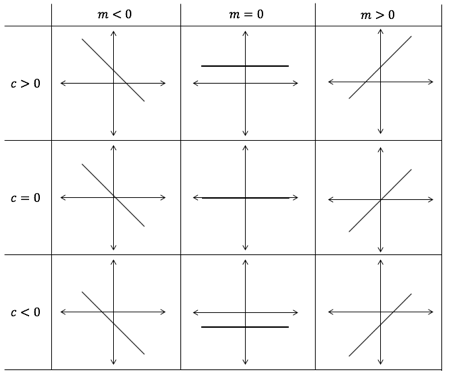
   1. As we change the value of [latex]\scriptsize c[/latex], the graph moves up and down. When we increase the value of [latex]\scriptsize c[/latex], we move the graph up. When we decrease the value of [latex]\scriptsize c[/latex], we move the graph down.
   2. The value of [latex]\scriptsize c[/latex] in [latex]\scriptsize y=mx+c[/latex] is the point where the graph cuts or intercepts the y-axis. We call this point the y-intercept.
   3. As we change the value of [latex]\scriptsize m[/latex], we change the slope or gradient of the graph.
   4. A large value of [latex]\scriptsize m[/latex] gives a graph with a very steep slope. A small value of [latex]\scriptsize m[/latex] gives a graph with a very shallow slope.
   5. When [latex]\scriptsize m[/latex] is positive, the graph slopes up from left to right. When [latex]\scriptsize m[/latex] is negative the graph slopes down from left to right.
   6. When [latex]\scriptsize m=0[/latex], the graph is a flat horizontal line. When [latex]\scriptsize m=0[/latex], the function becomes [latex]\scriptsize y=c[/latex]. In other words, it makes no difference what input value we choose, the output value will always be [latex]\scriptsize c[/latex]. Thus, all the points on the graph will have a y-coordinate of [latex]\scriptsize c[/latex].

We learnt a lot from that last activity. Let’s look at two different ways to sketch a linear function.

Any two points

One way we have of sketching a linear function is to find and plot any two points. We can do this by choosing any two input values and then finding out what the corresponding function or output values are. For example, if we had [latex]\scriptsize q(x)=2x-1[/latex], we might choose [latex]\scriptsize x=1[/latex] and [latex]\scriptsize x=2[/latex]. Then [latex]\scriptsize q(1)=2(1)-1=1[/latex] and [latex]\scriptsize q(2)=2(2)-1=3[/latex]. We would then plot the points [latex]\scriptsize (1,1)[/latex] and [latex]\scriptsize (2,3)[/latex] and join them with a straight line as shown in Figure 9.

Dual-intercept method

However, we can simplify things if we plot the points where the graph intercepts with the axes. Where the graph crosses the x-axis, this is the x-intercept and the y-coordinate of the point is zero. Where the graph crosses the y-axis, this is the y-intercept and the x-coordinate of the point is zero.

So, plotting [latex]\scriptsize q(x)=2x-1[/latex]:

• x-intercept (make [latex]\scriptsize y=0[/latex]): [latex]\scriptsize 0=2x-1 \therefore 2x=1 \therefore x=\displaystyle \frac{1}{2}[/latex]. Therefore, the point to plot is [latex]\scriptsize (\displaystyle \frac{1}{2},0)[/latex].
• y-intercept (make [latex]\scriptsize x=0[/latex]): [latex]\scriptsize q(0)=2(0)-1=-1[/latex]. Therefore, the point is [latex]\scriptsize (0,-1)[/latex].

If we plot these points and join them with a straight line, we get the graph in Figure 10 which is identical to the graph in Figure 9 because we plotted the same function.

Can you see why we can only look at the value of [latex]\scriptsize c[/latex] as a short-cut for finding the y-intercept? Can you also see why it is called the dual-intercept method for sketching a linear function? We find both intercepts.

The gradient of a straight line graph

We have already seen that when the linear function is in the form [latex]\scriptsize y=mx+c[/latex], the value of [latex]\scriptsize c[/latex] immediately tells us what the y-intercept of the graph is. The value of [latex]\scriptsize m[/latex] tells us what the slope or gradient of the graph is. The bigger the value of [latex]\scriptsize m[/latex], the steeper the graph.

Here is a summary of what we know so far.

Take note!

Remember, that we sometimes write the standard form of the linear function as [latex]\scriptsize y=ax+q[/latex]. In this case [latex]\scriptsize q[/latex] tells us what the y-intercept is and the value of [latex]\scriptsize a[/latex] gives us the gradient of the graph. Let’s take a closer look at the gradient.

This activity will help you understand what the gradient of a straight line is and how to measure it.

Activity 1.4: The gradient of a straight line graph

Time required: 30 minutes

What you need:

• a pen or pencil
• blank paper or a notebook
• an internet connection (optional)

What to do:

1. Figure 11 is a graph of the function [latex]\scriptsize y=2x+1[/latex]. Look at Figure 11 and answer the following questions.
   

   

   1. What is the length of the horizontal purple line? How does this length relate to the difference in the x-coordinates of points A and B?
   2. What is the length of the vertical green line? How does this length relate to the difference in the x-coordinates of points A and B?
   3. Calculate the value of [latex]\scriptsize \displaystyle \frac{\text{length of green line}}{\text{length of purple line}}[/latex]. What characteristic of the graph does this value measure?
   4. Pick any two other points on the graph and again measure the difference in their x- and y-coordinates in order to work out the same ratio of [latex]\scriptsize \displaystyle \frac{\text{length of green line}}{\text{length of purple line}}[/latex].
   5. What characteristic of the graph is this value of [latex]\scriptsize \displaystyle \frac{\text{length of green line}}{\text{length of purple line}}[/latex] equal to?
2. If you have an internet connection, open the gradient of a straight line graph interactive simulation.
   

Here you will find a linear function of the form [latex]\scriptsize y = mx+c[/latex] with sliders so that you can change the values of [latex]\scriptsize m[/latex] and [latex]\scriptsize c[/latex]. Set the graph to represent the function [latex]\scriptsize y=\displaystyle \frac{1}{2}x-1[/latex]. Drag the purple point to [latex]\scriptsize (2;0)[/latex] and the green point to [latex]\scriptsize (4;1)[/latex].

By looking at the equation of the function, what do you expect the value of [latex]\scriptsize \displaystyle \frac{\text{length of green line}}{\text{length of purple line}}[/latex] to be? Measure the length of the lines and calculate the value. Is it what you expected? Now move either or both points to other places on the graph and recalculate the value of [latex]\scriptsize \displaystyle \frac{\text{length of green line}}{\text{length of purple line}}[/latex]. Do you get the same answer? Why do you think this is?

Now, set the graph to represent [latex]\scriptsize y=-2x+1[/latex] and move the purple point to [latex]\scriptsize (-1;3)[/latex] and the green point to [latex]\scriptsize (1;-1)[/latex]. What do you expect the value of [latex]\scriptsize \displaystyle \frac{\text{length of green line}}{\text{length of purple line}}[/latex] to be? Measure the length of the lines and calculate the value. Is it what you expected?

What changes to your calculations did you have to make to arrive at the answer of [latex]\scriptsize -2[/latex] for [latex]\scriptsize \displaystyle \frac{\text{length of green line}}{\text{length of purple line}}[/latex]? Move the green and purple points to any other parts of the graph and recalculate the value of [latex]\scriptsize \displaystyle \frac{\text{length of green line}}{\text{length of purple line}}[/latex]. Do you still get the same answer?

Change the value of [latex]\scriptsize m[/latex] to any other value you like and verify that you are able to use the same method as above to measure or calculate the gradient.

Write a general expression that will allow you to measure the gradient of any straight-line graph between any two points on the line.

What did you find?

In Question 1, we looked at Figure 11 showing the graph of [latex]\scriptsize y=2x+1[/latex]. The length of the purple line was two units. This was the difference between the x-coordinates of points A and B ([latex]\scriptsize \text{(x-coordinate of B)}–\text{(x-coordinate of A)}=2-1=1[/latex]). The length of the green line was two units and was the difference between the y-coordinates of the points A and B ([latex]\scriptsize \text{(y-coordinate of B)}–\text{(y-coordinate of A)}=5-3=2[/latex]).

Therefore [latex]\scriptsize \displaystyle \frac{\text{length of green line}}{\text{length of purple line}}=\displaystyle \frac{2}{1}=2[/latex]. This is a measure of how steep the graph is; in other words, its gradient.

No matter which other points we choose, the value of [latex]\scriptsize \displaystyle \frac{\text{length of green line}}{\text{length of purple line}}[/latex] stays [latex]\scriptsize 2[/latex]. For example, if we chose the points [latex]\scriptsize (0;1)[/latex] and [latex]\scriptsize (3;7)[/latex] , the value of [latex]\scriptsize \displaystyle \frac{\text{length of green line}}{\text{length of purple line}}[/latex] would be:

[latex]\scriptsize \displaystyle \frac{\text{length of green line}}{\text{length of purple line}}=\displaystyle \frac{7-1}{3-0}\displaystyle \frac{6}{3}=2[/latex]

The value of [latex]\scriptsize \displaystyle \frac{\text{length of green line}}{\text{length of purple line}}[/latex] is the same as the value of [latex]\scriptsize m[/latex] in the equation of the function. We know that [latex]\scriptsize m[/latex] describes the gradient of the graph. Therefore [latex]\scriptsize \displaystyle \frac{\text{length of green line}}{\text{length of purple line}}[/latex] is a measure of the gradient of the graph as well.

If you were able to practise using the gradient of a straight line graph interactive simulation of the function [latex]\scriptsize y=\displaystyle \frac{1}{2}x-1[/latex], you would have found that no matter where you dragged the green and purple points to, the value of [latex]\scriptsize \displaystyle \frac{\text{length of green line}}{\text{length of purple line}}[/latex] was always equal to the value of [latex]\scriptsize m[/latex] in the equation of the function which was [latex]\scriptsize \displaystyle \frac{1}{2}[/latex].

For the function [latex]\scriptsize y=-2x+1[/latex], the same thing was true. To find the value of [latex]\scriptsize \displaystyle \frac{\text{length of green line}}{\text{length of purple line}}[/latex] between the points [latex]\scriptsize (-1;3)[/latex] and [latex]\scriptsize (1;-1)[/latex] our calculations were as follows:

[latex]\scriptsize \displaystyle \frac{\text{length of green line}}{\text{length of purple line}}=\displaystyle \frac{3-(-1)}{-1-1}=\displaystyle \frac{4}{-2}=-2[/latex]

Or

[latex]\scriptsize \displaystyle \frac{\text{length of green line}}{\text{length of purple line}}=\displaystyle \frac{-1-3)}{1-(-1)}=\displaystyle \frac{-4}{2}=-2[/latex]

It does not matter in which order we subtracted the coordinates so long as we always used the same order.

If we have any two points on a straight line, for example [latex]\scriptsize (x_{1};y_{1})[/latex] and [latex]\scriptsize (x_{2};y_{2})[/latex], then we can calculate the gradient of the straight line as follows:

[latex]\scriptsize m=\displaystyle \frac{y_{2}-y_{1}}{x_{2}-x_{1}}[/latex]

It does not matter which is point 1 and which is point 2, so long as you subtract the coordinates in the same order.

The expression for the gradient of a straight line covered above is important and you will need to use it often in many different scenarios. Other ways you may see the gradient of a straight line expressed are:

[latex]\scriptsize \displaystyle \frac{\text{rise}}{\text{run}}[/latex] or [latex]\scriptsize \displaystyle \frac{\text{change in }y}{\text{change in }x}[/latex] or [latex]\scriptsize \displaystyle \frac{\text{vertical change}}{\text{horizontal change}}[/latex]

All these mean the same thing. When moving from left to right between any two points, how much the graph goes up (or down) from the one point to the next, divided by how far the graph moves to the right to achieve this up or down change.

Now that we know what gradient is and how to measure it, we can look at another way to sketch linear functions.

Example 1.5

1. Sketch the function [latex]\scriptsize t(x)=1-2x[/latex] by finding the y-intercept and then measuring out the gradient to find another point on the line.
2. Sketch the linear function [latex]\scriptsize r(x)[/latex] that has a y-intercept at [latex]\scriptsize (0,3)[/latex] and a gradient of [latex]\scriptsize \displaystyle \frac{3}{2}[/latex].
3. A straight line is parallel to the line [latex]\scriptsize 3y+4x-7=0[/latex] and passes through the point [latex]\scriptsize (0,-2)[/latex]. What is the equation of the line? Sketch the line. Note: Parallel lines have the same gradient.

Solution

1. .
   First, we need to get our function into standard form.[latex]\scriptsize t(x)=-2x+1[/latex]
   .
   Now we can see that the y-intercept is the point [latex]\scriptsize (0,1)[/latex] and the gradient is [latex]\scriptsize -2[/latex] or [latex]\scriptsize \displaystyle \frac{-2}{1}[/latex]. This means that for every one unit we move to the right, we have to move two units down. Starting at the y-intercept, we measure out the gradient – one unit right and then two units down. We mark this point and then join our two points with a straight line (see Figure 12).
   .

   

   .
   Note: It is important that when measuring a gradient, you always move from left to right (i.e. in the positive horizontal direction) and then up or down depending on whether the gradient is positive or negative. In the case above, if we moved from right to left (the negative horizontal direction), we would have to go up. Going down (in the negative vertical direction) would have measured a gradient of [latex]\scriptsize \displaystyle \frac{-2}{-1}=\displaystyle \frac{2}{1}[/latex] not [latex]\scriptsize \displaystyle \frac{-2}{1}[/latex].

2. .
   We know that the gradient of the line is [latex]\scriptsize \displaystyle \frac{3}{2}[/latex]. In other words, if we move two units to the right, we have to move three up. The y-intercept is the point [latex]\scriptsize (0,3)[/latex], so this is a good place from which to start measuring the gradient. Figure 13 shows the graph.
   .

   

3. .
   We are told that our graph is parallel to [latex]\scriptsize 3y+4x-7=0[/latex]. Therefore, it has the same gradient. To find the gradient, we have to get the parallel line into standard form.

[latex]\scriptsize \begin{align*} 3y+4x-7&=0\\ \therefore 3y&=-4x+7\\ \therefore y&=\displaystyle \frac{-4}{3}x+\displaystyle \frac{7}{3} \end{align*}[/latex]

The gradient of the graph is [latex]\scriptsize \displaystyle \frac{-4}{3}[/latex]. We are also told that it passes through the point [latex]\scriptsize (0;-2)[/latex]. So, starting at the point [latex]\scriptsize (0;-2)[/latex] (which is the y-intercept but could really be any point on the line), we measure out the gradient – three units to the right and then 4 units down. The graph is shown in Figure 14.

Exercise 1.3

Use any method to plot the following linear functions on the same set of axes.

1. [latex]\scriptsize 2y=3x-1[/latex]
2. [latex]\scriptsize y=x-3[/latex]
3. [latex]\scriptsize 2x-3y=12[/latex]
4. [latex]\scriptsize y+3x-3=1[/latex]

The full solutions are at the end of the unit.

Domain and range

Have you wondered yet why we sketch straight line graphs by just finding any two points and then join them with a solid line? Think about the function [latex]\scriptsize f(x)=3x-2[/latex]. Is there any value of [latex]\scriptsize x[/latex] that we cannot put into the equation? Is there any value of [latex]\scriptsize y[/latex] that the function cannot be equal to?

The answer to both questions is ‘no’. We say that the domain (remember, this is just a fancy name for the set of all input values) is all real numbers. Similarly, the range (the set of all output values) is also all real numbers. If we were to plot all the possible input and output pairs for the function on the same set of axes, there would be so many points that they would blur together and form a solid line.

But we can restrict what input values a function is allowed to have and, in so doing, restrict the output values that a function can produce. Sometimes the nature of the function itself automatically restricts what input values are allowed. Look at this example:

[latex]\scriptsize t(x)=\displaystyle \frac{x+3}{x-1}[/latex]

We know that we are never allowed to divide by zero which means the denominator in this function may never be zero. This means that [latex]\scriptsize x\neq1[/latex]. In this case, the function is allowed to take any real number as an [latex]\scriptsize x[/latex] value except [latex]\scriptsize 1[/latex]. We can write this domain formally using set notation like this:

Domain: [latex]\scriptsize \{x:x\in \mathbb{R},x\neq1\}[/latex]

Here is another domain: [latex]\scriptsize \{x:x\in \mathbb{R},-2\leq x\lt 5\}[/latex]. This one says that the domain is all the real numbers between [latex]\scriptsize -2[/latex] and [latex]\scriptsize 5[/latex], including [latex]\scriptsize -2[/latex] but not including [latex]\scriptsize 5[/latex].

We could also write this slightly less formally using interval notation as [latex]\scriptsize [-2;5)[/latex]. The square bracket tells us that the domain includes [latex]\scriptsize -2[/latex] and the round bracket tells us that it does not include [latex]\scriptsize 5[/latex]. When using interval notation, we assume that the interval contains all real numbers.

Generally, unless there is a specific restriction imposed, linear functions can take any real number as an input and it is possible to generate any real number as an output. Therefore, the Domain and Range of linear functions is almost always:

• Domain: [latex]\scriptsize \{x:x\in \mathbb{R}\}[/latex] or [latex]\scriptsize (-\infty;\infty)[/latex] – the round brackets indicate that the domain does not include [latex]\scriptsize -\infty[/latex] or [latex]\scriptsize \infty[/latex].
• Range: [latex]\scriptsize \{x:x\in \mathbb{R}\}[/latex] or [latex]\scriptsize (-\infty;\infty)[/latex] – the round brackets indicate that the range does not include [latex]\scriptsize -\infty[/latex] or [latex]\scriptsize \infty[/latex].

Exercise 1.4

1. Write the following in set notation:
   1. [latex]\scriptsize (-\infty; 6)[/latex]
   2. [latex]\scriptsize [-12; 13)[/latex]
   3. [latex]\scriptsize (-\sqrt{3}; \infty)[/latex]
2. Write the following in interval notation:
   1. [latex]\scriptsize \{p:p\in \mathbb{R}\}[/latex]
   2. [latex]\scriptsize \{k:k\in \mathbb{R},k\gt\displaystyle \frac{2}{5}\}[/latex]
   3. [latex]\scriptsize \{r:r\in \mathbb{R},13\lt r \leq 42\}[/latex]

The full solutions are at the end of the unit.

Finding the equation of a linear function

We know how to draw a graph for a linear function if we know its equation. But can we find its equation if, all we have is its graph?

Example 1.6

1. Find the equation of the function shown in the graph below.
   
2. A linear function, [latex]\scriptsize s(x)[/latex], passes through the points [latex]\scriptsize (-6,1)[/latex] and [latex]\scriptsize (2,-3)[/latex]. What is its equation?
3. [latex]\scriptsize g(x)[/latex] is parallel to [latex]\scriptsize 3y-5x+6=0[/latex] and passes through [latex]\scriptsize (-2,-\displaystyle \frac{3}{2})[/latex]. What is the equation of [latex]\scriptsize g(x)[/latex]?

Solution

1. .
   The graph passes through the points [latex]\scriptsize (0,2)[/latex] and [latex]\scriptsize (1,-1)[/latex] . We can see that [latex]\scriptsize (0,2)[/latex] is the y-intercept, therefore we know that [latex]\scriptsize c=2[/latex]. We can use these two points to find the gradient.
   .
   [latex]\scriptsize m=\displaystyle \frac{y_{2}-y_{1}}{x_{2}-x_{1}}=\displaystyle \frac{2-(-1)}{0-1}=\displaystyle \frac{3}{-1}=-3[/latex]
   .
   Therefore, the equation of the function is [latex]\scriptsize y=-3x+2[/latex].
2. .
   We are told that the function passes through points [latex]\scriptsize (-6,1)[/latex] and [latex]\scriptsize (2,-3)[/latex].
   [latex]\scriptsize m=\displaystyle \frac{y_{2}-y_{1}}{x_{2}-x_{1}}=\displaystyle \frac{-3-1}{2-(-6)}=\displaystyle \frac{-4}{8}=\displaystyle \frac{-1}{2}[/latex]
   .
   Therefore, [latex]\scriptsize s(x)=-\displaystyle \frac{1}{2}x+q[/latex]. To find the value of [latex]\scriptsize q[/latex], we substitute either point into the equation of [latex]\scriptsize s(x)[/latex]. For example, we know that [latex]\scriptsize s(2)=-3[/latex].
   .
   [latex]\scriptsize \begin{align*} s(2)&=2(-\displaystyle \frac{1}{2})+q=-3\\ \therefore -1+q&=-3\\ \therefore -1+3&=-q\\ \therefore q&=-2 \end{align*}[/latex]
   .
   So [latex]\scriptsize s(x)=-\displaystyle \frac{1}{2}x-2[/latex]
3. .
   [latex]\scriptsize g(x)[/latex] is parallel to [latex]\scriptsize 3y-5x+6=0[/latex]. Writing [latex]\scriptsize 3y-5x+6=0[/latex] in standard form, we get
   .
   [latex]\scriptsize \begin{align*} 3y-5x+6&=0\\ \therefore 3y&=5x-6\\ \therefore y&=\displaystyle \frac{5}{3}x-2 \end{align*}[/latex]
   .
   Therefore [latex]\scriptsize g(x)=\displaystyle \frac{5}{3}x+q[/latex]. We are also told that [latex]\scriptsize g(x)[/latex] passes through [latex]\scriptsize (-2;-\displaystyle \frac{3}{2})[/latex]. Therefore, [latex]\scriptsize g(-2)=\displaystyle \frac{3}{2}[/latex]
   .
   [latex]\scriptsize \begin{align*} g(-2)&=\displaystyle \frac{5}{3}(-2)+q=\displaystyle \frac{3}{2}\\ \therefore \displaystyle \frac{-10}{3}+q&=\displaystyle \frac{3}{2}\\ \therefore -20+6q&=9\\ \therefore 6q&=29\\ \therefore q&=\displaystyle \frac{29}{6} \end{align*}[/latex]
   .
   So finally we know that [latex]\scriptsize g(x)=\displaystyle \frac{5}{3}x+\displaystyle \frac{29}{6}[/latex] .

Summary

In this unit you have learnt the following:

• That a function is a mathematical relationship between inputs and outputs that maps each input to one, and only one, output.
• The difference between a function and a relation.
• The standard form of a linear function is [latex]\scriptsize y=mc+c[/latex] (or [latex]\scriptsize y= ax+q[/latex]).
• The effect of [latex]\scriptsize m[/latex] and [latex]\scriptsize c[/latex] (or [latex]\scriptsize a[/latex] and [latex]\scriptsize q[/latex]) on the graph of a linear function.
• What we mean by the domain and range of a linear function and how to represent these in set and interval notation.
• How to plot the graph of a linear function using any two points, the dual-intercept method and the gradient-intercept method.
• How to find the equation of a linear function.

Unit 1: Assessment

Suggested time to complete: 40 minutes

1. Write the following linear functions in standard form.
   1. [latex]\scriptsize 2y+3x=1[/latex]
   2. [latex]\scriptsize y+2x-3=1[/latex]
2. Determine the x- and y-intercepts of [latex]\scriptsize x+2y-2=0[/latex].
3. Determine the equation of the following linear function.
   
4. Are the following statements true or false?
   1. The gradient of [latex]\scriptsize 2y=3x-1[/latex] is [latex]\scriptsize 3[/latex].
   2. The gradient of [latex]\scriptsize 2-y=2x-1[/latex] is [latex]\scriptsize -2[/latex].
   3. The y-intercept of [latex]\scriptsize 2y+3x=6[/latex] is [latex]\scriptsize 6[/latex].
5. [latex]\scriptsize f(x)=3-3x[/latex] and [latex]\scriptsize g(x)-1=\displaystyle \frac{1}{3}x[/latex] .
   1. Sketch both graphs on the same set of axes using any method. Make sure to label your axes and functions.
   2. Find the point where the graphs cross or intersect.

The full solutions are at the end of the unit.

Unit 1: Solutions

Exercise 1.1

1. Moving a vertical line across the graph from left to right, at no point does the line cut the graph more than once. Therefore, the graph represents a function.
2. Moving a vertical line across the graph from left to right, at no point does the line cut the graph more than once. Therefore, the graph represents a function.
3. Moving a vertical line across the graph from left to right, at no point does the line cut the graph more than once. Therefore, the graph represents a function.
4. For input values between [latex]\scriptsize -4[/latex] and [latex]\scriptsize 4[/latex], a vertical line will cut the graph more than once. Therefore, the graph does not represent a function.
5. For input values less than about [latex]\scriptsize 1.9[/latex] a vertical line will cut the graph more than once. Therefore, the graph does not represent a function.
6. Moving a vertical line across the graph from left to right, at no point does the line cut the graph more than once. Therefore, the graph represents a function.

Back to Exercise 1.1

Exercise 1.2

1. [latex]\scriptsize f(x)=2x-3[/latex]
   1. table of values
      

      [latex]\scriptsize x[/latex]	[latex]\scriptsize -2[/latex]	[latex]\scriptsize -1[/latex]	[latex]\scriptsize 0[/latex]	[latex]\scriptsize 1[/latex]	[latex]\scriptsize 2[/latex]
      [latex]\scriptsize y[/latex]	[latex]\scriptsize -7[/latex]	[latex]\scriptsize -5[/latex]	[latex]\scriptsize -3[/latex]	[latex]\scriptsize -1[/latex]	[latex]\scriptsize 1[/latex]

   2. mapping diagram
      
   3. graph
      
2. [latex]\scriptsize f(x)=x^2-2[/latex], [latex]\scriptsize g(x)=x-3[/latex] and [latex]\scriptsize k(x)=3[/latex].
   1. [latex]\scriptsize f(-1)=(-1)^2-2=1-2=-1[/latex]
   2. [latex]\scriptsize f(-6)=(-6)^2)-2=36-2=34[/latex]
   3. [latex]\scriptsize k(2)=3[/latex]
   4. [latex]\scriptsize k(-1)+f(3)-g(7)=3+[(3)^2-2]-[(7)-3]=3+7-4=6[/latex]
   5. [latex]\scriptsize g(f(4))[/latex]
      [latex]\scriptsize f(4)=(4)^2-2=16-2=14[/latex]
      [latex]\scriptsize g(14)=14-3=11[/latex]
3. Cost of petrol: [latex]\scriptsize P=15.61L[/latex]; cost of diesel: [latex]\scriptsize D=13.47L[/latex] where [latex]\scriptsize L[/latex] is the amount in litres:
   1. [latex]\scriptsize P=15.61\times30=\text{R}468.30[/latex]
   2. [latex]\scriptsize D(35)=13.47\times35=\text{R}471.45[/latex]
   3. .
      [latex]\scriptsize \begin{align*} P=15.61\ L&=300\\ \therefore L&=\displaystyle \frac{300}{15.61}\\ \therefore L&=19.11~\text{l} \end{align*}[/latex]
   4. .
      [latex]\scriptsize \begin{align*} D=13.47\ L&=450\\ \therefore L&=\displaystyle \frac{450}{13.47}\\ \therefore L&=33.41~\text{l} \end{align*}[/latex]
   5. Let price difference be the function [latex]\scriptsize Q[/latex]. Then [latex]\scriptsize Q=P-D=15.61L-13.47L=L(15.61-13.47)=2.14L[/latex].

Back to Exercise 1.2

Exercise 1.3

Back to Exercise 1.3

Exercise 1.4

1. .
   1. [latex]\scriptsize \{x:x\in \mathbb{R},x\lt6\}[/latex]
   2. [latex]\scriptsize \{x:x\in \mathbb{R},-12\lt x\lt13\}[/latex]
   3. [latex]\scriptsize \{x:x\in \mathbb{R},x\gt-\sqrt{3}\}[/latex]
2. .
   1. [latex]\scriptsize (-\infty,\infty)[/latex]
   2. [latex]\scriptsize (\displaystyle \frac{2}{5},infty)[/latex]
   3. [latex]\scriptsize (13,42][/latex]

Back to Exercise 1.4

Unit 1: Assessment

1. .
   1. .
      [latex]\scriptsize \begin{align*} 2y+3x&=1\\ \therefore 2y&=-3x+1\\ \therefore y&=-\displaystyle \frac{3}{2}x+\displaystyle \frac{1}{2} \end{align*}[/latex]
   2. .
      [latex]\scriptsize \begin{align*} y+2x-3&=1\\ \therefore y&=-2x+4\\ \end{align*}[/latex]
2. .
   [latex]\scriptsize x+2y-2=0[/latex]
   x-intercept (let [latex]\scriptsize y=0[/latex]):
   [latex]\scriptsize \begin{align*} x+2(0)-2&=0\\ \therefore x&=2 \end{align*}[/latex]
   [latex]\scriptsize \therefore \text{the x-intercept is } (2,0)[/latex]
   .
   y-intercept (let [latex]\scriptsize x=0[/latex]):
   [latex]\scriptsize \begin{align*} 0+2y-2&=0\\ \therefore 2y&=2\\ \therefore y&=1 \end{align*}[/latex]
   [latex]\scriptsize \therefore \text{the x-intercept is } (0,1)[/latex]
3. The graph passes through the point [latex]\scriptsize (0,-1)[/latex] and [latex]\scriptsize (1,2)[/latex]. Therefore, the y-intercept (the value of [latex]\scriptsize c[/latex] is [latex]-1[/latex].
   [latex]\scriptsize m=\displaystyle \frac{y_2-y_1}{x_2-x_1}=\displaystyle \frac{2-(-1)}{1-0}=\displaystyle \frac{3}{1}=3[/latex]
   Therefore, the equation of the line is [latex]\scriptsize y=3x-1[/latex].
4. .
   1. .
      [latex]\scriptsize \begin{align*} 2y&=3x-1\\ \therefore y&=\displaystyle \frac{3}{2}-\displaystyle \frac{1}{2}\\ \therefore m=\displaystyle \frac{3}{2} \end{align*}[/latex]
      Therefore, the statement is false.
   2. .
      [latex]\scriptsize \begin{align*} 2-y&=2x-1\\ \therefore y&=-2x+3\\ \therefore m&=-2 \end{align*}[/latex]
      Therefore, the statement is true.
   3. .
      [latex]\scriptsize \begin{align*} 2y+3x=6\\ \therefore 2y&=-3x+6\\ \therefore y&=-\displaystyle \frac{3}{2}+3 \therefore c=3 \end{align*}[/latex]
      Therefore, the statement is false.
5. .
   1. .
      Given [latex]\scriptsize f(x)=3-3x[/latex] and [latex]\scriptsize g(x)-1=\displaystyle \frac{1}{3}x[/latex].
      [latex]\scriptsize f(x)=3-3x[/latex]
      x-intercept (let [latex]\scriptsize y=0[/latex]):
      [latex]\scriptsize \begin{align*} 0&=3-3x\\ \therefore 3x&=3\\ \therefore x&=1 \end{align*}[/latex]
      y-intercept (let [latex]\scriptsize x=0[/latex]):
      [latex]\scriptsize \begin{align*} y&=3-3(0)\\ \therefore y&=3 \end{align*}[/latex]
      .
      [latex]\scriptsize g(x)-1=\displaystyle \frac{1}{3}x[/latex]
      x-intercept (let [latex]\scriptsize y=0[/latex]):
      [latex]\scriptsize \begin{align*} 0-1&=\displaystyle \frac{1}{3}x\\ \therefore x&=-3 \end{align*}[/latex]
      y-intercept (let [latex]\scriptsize x=0[/latex]):
      [latex]\scriptsize \begin{align*} y-1&=\displaystyle \frac{1}{3}(0) \\ \therefore y&=1 \end{align*}[/latex]
      .
      
   2. .
      To find the point where the graphs intersect each other, we need to set [latex]\scriptsize f(x)=g(x)[/latex].
      [latex]\scriptsize f(x)=3-3x[/latex] and [latex]\scriptsize g(x)=\displaystyle \frac{1}{3}x+1[/latex]
      [latex]\scriptsize \begin{align*} f(x)&=g(x) &&\text{Setting the functions equal to each other will allow us find the }x\text{ co-ordinate of the point of intersection}\\ \therefore 3-3x&=\displaystyle \frac{1}{3}x+1\\ \therefore 9-9x&=x+3\\ \therefore -10x&=-6\\ \therefore x&=\displaystyle \frac{6}{10}=\displaystyle \frac{3}{5} \end{align*}[/latex]
      Now substitute [latex]\scriptsize x=\displaystyle \frac{4}{5}[/latex] in either function to find the y-coordinate of the point.
      [latex]\scriptsize \begin{align*} f(\displaystyle \frac{3}{5})&=3-3(\displaystyle \frac{3}{5})=3-\displaystyle \frac{9}{5}\\ \therefore f(\displaystyle \frac{3}{5})&=\displaystyle \frac{15-9}{5}=\displaystyle \frac{6}{5} \end{align*}[/latex]
      Therefore, the point of intersection is [latex]\scriptsize (\displaystyle \frac{3}{5},\displaystyle \frac{6}{5})[/latex] .

Back to Unit 1: Assessment